Logging data is almost as dangerous as logging trees; if you don’t do either the right way, the consequences could be undesirable. Below I will explain why we log data in OLS. Then I will discuss how to interpret the coefficient of a logged independent variable in an OLS model. The interpretation is not as straight forward as it normally is in a linear OLS model. If it is not done carefully, the results of the model may be difficult to understand.
More following the jump….
Logging in OLS
OLS assumes there is a linear relationship between X and Y. However, sometimes our theory tells us that there is a non-linear relationship between X and Y. For example, we may expect parties to centralize more drastically when their membership increases from 0 to 1000, but centralize at a slower rate when their membership increases from 1000 to 2000. In both cases, the membership changes by 1000 people, but the effect on how much to centralize is not the same. In this case, we may expect that changes in lower values of X result in large changes in Y, while changes at higher levels of X result in smaller changes in Y.
Graph 1 below demonstrates the above aforementioned relationship between X and Y.
Graph 1: Relationship between X and Y

Running a model between two variables in OLS that have a non-linear relationship is dangerous. The model’s significance tests rely on the assumption the error term is random. When it is not random, such as in cases where the relationship between X and Y is non-linear, then we cannot trust the results.
We can overcome the non-linearity problem between X and Y by logging X. Graph 2 demonstrates that after logging X, the relationship between X (X-logged in this case) and Y becomes linear.
Graph 2: Logged X turns it into a linear relationship with Y

I ran several models in STATA to demonstrate how not logging your independent variable could affect the OLS results if it should be logged. I created a dependent variable, Y, which was function of the logged X, and a random component. Below are results from regressing X on Y and X-logged on Y. As you can see below, the first model accurately predicts the direction and significance of the relationship between X and Y. However, the R-squared is significantly lower in the first model than the x-logged model. Further, the data we normally use is not as accurate as the data in this model, so we should expect worse results than the ones reported here if we don’t log our data when we should.
Now for the extremely important note about using a logged independent variable is OLS: We should interpret the coefficients in both models differently. In the first model, we simply interpret the coefficient to mean that a one unit change in X will have a 0.0000302 unit change in Y. In the second model, we could interpret the coefficient to demonstrate the relationship between X-logged and Y but that does not tell us the relationship between X and Y. We can actually figure out how what the relationship between X and Y is from these results. The coefficient tells us how much Y will change given a 1% change in X. So in this example, since the coefficient is 1.009192, Y will change by (1.009192/100) units, or 0.0109129 units when X changes by 1%. Why is this case? It’s in the math (this is from Gujarati 2003, 181-182; also see why you divide the coefficient by 100 in the comment below):
Y = β1 + β2 ln X1 + µ1
dy/dx = β2 (1/x)
Or in other words…
∆Y /∆ X = β2 (1/x)
∆Y = β2 (∆ X/x)
So when using a logged independent variable in OLS, we should make sure to be careful about explaining what the coefficient exactly means. The direction and significance are interpreted the same way it is in any old OLS model, but figuring out what the relationship is between X and Y is different. I ran across a recent article in a Political Science journal that interpreted a logged coefficient as the effect of X-logged on Y. Although this is mathematically correct, more information between X and Y could have been discovered had they interpreted the coefficient differently.
Table 1: OLS Regression of Y and X
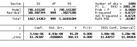
Table 2: OLS Regression of Y and X-logged

I ran across this post and thought that it might need some clarification. While the author is correct about the effect of a 1% change, she misinterprets how 1% is entered into the equation. In the log independent variable, a 1% change is entered into the equation as .01. Therefore, as Gujarati (1995, p. 172 (I know old edition)) states in the indented text, “[W]hen regressions like (6.5.11) are estimated by OLS, multiply the value of the estimated slope coefficient, B2, by .01, or, what amounts to the same thing, divide it by 100.” So, in the example above, the proper interpretation is that a 1% change in X will result in a .0109129% change in the dependent variable. I know there is a lot of confusion about this, and this is the first link that comes up from google, so I thought this might be helpful.
Thanks for the note. I did mistake 0.01 for 1. However, I think the intrepretation may be slightly different than what was stated.
The left hand side of the equation (changed in Y) represents a numeric change, not a percentage change. Hence, I think the correct interpretation should be:
A 1% changed in x causes a 0.0109129 change in y. (Not a % change in Y)
Does this seem correct?
Could we consider the same interpretation also for a negative binomial regression with logged x?
Thank You
I think you guys are correct, the difference is about whether the model is Log-lo(Double logged model or semi logged model .Its important to understand that logging variables is not for fun, it is meant to smooth out the non linearity in the first place(Gujarati, 2005 P.53 & 567)when that is done, interpreting is not because of the log alone but the type of log in place i.e Log-log model or the semi log model.If its log-log model(DV and IVS are logged), the interpretation of percentage change or a unit change affects both the DVs and the IVs but if is a semi log, the slope coefficient(i.e B2) now measure the relative change or elasticity of the DV(Y); that is , relative change in the regressand in relation to absolute change in the regressor.My take anyway.Thanks